ResNet#
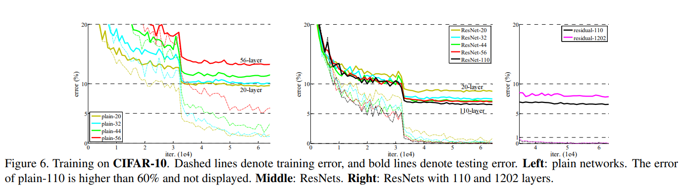
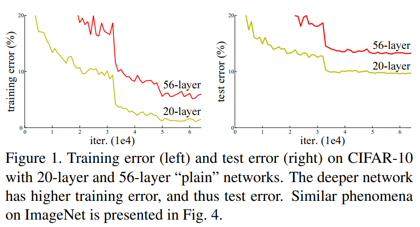
딥러닝에서 신경망이 깊어지면 깊어질수록 모형의 성능은 더 좋아진다. 하지만 모형을 학습하는 방법이 어렵다는 것도 알려진 사실이다. 레이어가 깊어질 수록 모형 학습과저에서 발생하는 대표적인 문제들은 기울기의 소실/폭발(problem of vanishing/exploding gradients)이다. 이를 해결하기 위해 다양한 방법이 제안되었다. 초기화, 정규화 계층 등. ResNet 연구팀은 학습과정 뿐만 아니라 성능 저하 문제(degradation problem)을 깊이 고찰한다. 이는 계층이 깊어질수록 정확도(accuracy)가 떨어지는 문제이다. 이는 과적합(overfitting)이 아닌 문제로 과적합이면 깊은 레이어에서 학습 정확도는 높고 테스트 정확도는 낮아야하는데 둘다 낮기 때문이다.
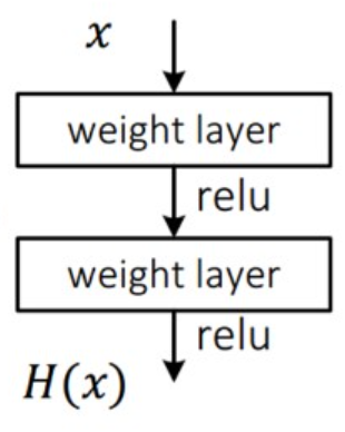
ResNet 연구팀은 성능 저하 문제는 모든 모형에 최적하기 쉽지 않다고 생각해 얕은 구조와 더 깊은 구조를 비교하고자 했다. 일반적인 합성곱 신경망의 경우 입력 \(x\)를 받아 두 개의 가중치 레이어를 거쳐 출력 \(H(x)\)를 거쳐 다음 레이어의 입력으로 사용된다.
ResNet 연구팀은 레이어의 입력을 출력 단계에 연결시키는 skip connection을 사용한다.
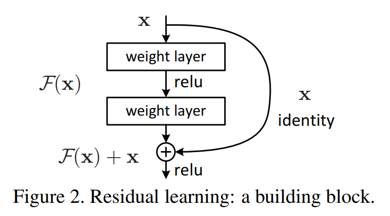
출력 단계에서 \(H(x)\)가 \(F(x)+x\)로 변경되었다. 단순히 가중치 레이어에서 나온 결과물을 입력 데이터와 더한 것일 뿐인데 성능이 매우 좋아졌다. 이유는 ResNet은 \(F(x)\)가 0이 되는 방향으로 학습하기 때문이다. \(F(x)=H(x)-x\)이고 \(F(x)\)를 학습한다는 것은 나머지(residual)을 학습한다고 볼 수 있다. 또한, \(x\)가 그대로 skip connection이 되기 때문에 연산 증가는 없고 \(F(x)\)가 몇 개의 레이어를 포함하게 할지 선택이 가능하다.
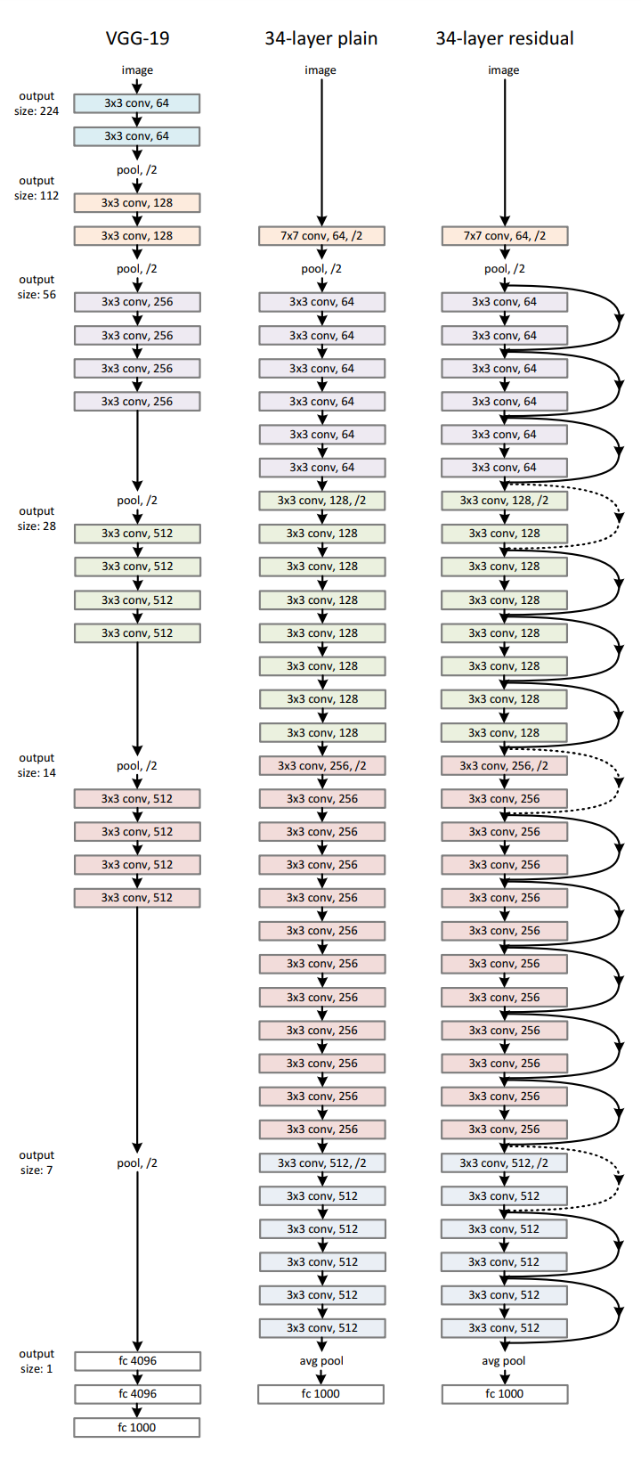
ResNet의 성능을 비교하기 위해 VGG19, 더 갚은 plain network, residual network를 설계하고 구조는 VGG를 참고해 설계하였다.
배치 정규화#
데이터셋을 딥러닝 모형을 학습하기 위해서 gradient descent 방법을 사용하고 graidient를 한번 업데이트 하기 위해 모든 학습 데이터를 사용한다. 하지만 한번에 모든 데이터셋을 넣어서 gradient를 구할 수 없기 때문에 일반적으로 대용량 데이터셋의 크기를 batch 단위로 나눠 학습한다. 그래서 사용하는 것이 stochastic gradient descent (SGD) 방법이고 SGD는 일부의 데이터만 사용한다.
따라서 학습 데이터 전체를 한번 학습하는 것을 Epoch이라 하고 gradient를 구하는 단위를 Batch라고 한다.
그러나 배치 단위로 학습하게 되면 발생하는 문제점 internal covariant shift이다. interval covariant shift는 학습과정에서 계층 별로 입력의 데이터 분포가 달라지는 현상을 뜻한다. 각 계층에서 입력 특징맵을 받고 그 특징 맵은 활성화 함수를 적용해 연산 전과 후의 데이터 분포가 달라질 수 있다. 배치 단위로 학습한다면 배치 단위간 데이터 분포의 차이가 더욱 심하다. 이를 개선하기 위해 배치 정규화(batch normalization)이 연구되었다. 배치 정규화(batch normalization)은 2015년 구글 Ioffe와 Szegedy의 Batch Normalization: Accelerating Deep Network Training by Reducing Internal Covariate Shift 논문으로 발표되었다.
배치 정규화는 학습 과정에서 배치마다 입력 데이터의 다양한 분포를 고려해 각 배치의 평균과 분산을 이용해 정규화하는 것이다. 목적은 각 계층마다 평균은 0, 표준 편차는 1인 분포로 조정한다.
\(\gamma\)는 스케일, \(\beta\)는 편향(bias)이다.
학습 단계#
학습 단계에서 배치 정규화는 배치별로 평균과 분산이 계산되어야 배치들이 정규 분포를 따르게 된다. 학습 단계에서 모든 특징에 정규화를 해주면 특징들이 동일한 스케일(scale)이 되어 학습률(learning rate) 결정에 유리해진다. 왜냐하면 특징의 스케일이 다르면 gradient descent 과정에서 gradient가 다르게 되고 같은 학습률에 대하여 가중치(weight)마다 반응하는 정도가 달라진다. 즉, gradient 편차가 크면 gradient가 큰 가중치에서 gradient exploding, 작으면 vanishing 현상에 발생한다.
일반적으로 배치 정규화는 활성화 함수 앞 단계에 적용하고 배치 정규화로 인해 가중치의 값은 평균 0, 분산1인 상태로 분포가 되지만, ReLU로 인해 음수에 해당하는 50%가 0이 되어 버려서 의미가 없어진다. 이를 예방하기 위해 \(\gamma\), \(\beta\)가 정규화 값이 곱해지고 더해져서 활성화 함수에 적용되더라도 기존의 음수 부분이 모두 0이 되지 않도록 방지해준다. 이 값은 학습을 통해 스스로 최적의 값으로 찾아간다. 또한, 배치 정규화의 편향으로 합성곱 신경망에서는 편향을 고려하지 않기도 한다.
추론 단계#
추론 과정에서 배치 정규화를 적용할 때 평균과 분산이 고정한다. 이 때 사용할 평균과 분산은 학습 과정에서 이동 평균(moving average) 또는 지수 평균(exponetial average)로 계산한 값이다. 학습했을 때 \(N\)개에 대한 평균 값을 고정 값으로 사용하는 것이다.
배치 정규화의 효과는 가중치 초기화(weight initialization)과 학습률(learning rate) 감소에 자유로워진다. 또한 regularization 효과가 있다. 배치로 평균과 분산이 변화되는 과정에서 분포가 바뀌면서 가중치에 영향을 주지만 배치 정규화는 가중치가 한쪽 방향으로만 학습되지 않기 때문에 제약화 효과가 있다. 따라서 과적합(overfitting) 문제에 강건(robust)해진다.
import torch
from torch import nn


def batch_norm(x, gamma, beta, moving_mean, moving_var, eps, momentum):
    if not torch.is_grad_enabled():
        x_hat = (x - moving_mean) / torch.sqrt(moving_var + eps)
    else:
        assert len(x.shape) in (2, 4)
        if len(x.shape) == 2:
            mean = x.mean(dim=0)
            var = ((x - mean) ** 2).mean(dim=0)
        else:
            mean = x.mean(dim=(0, 2, 3), keepdim=True)
            var = ((x - mean) ** 2).mean(dim=(0, 2, 3), keepdim=True)
        x_hat = (x - mean) / torch.sqrt(var + eps)
        moving_mean = momentum * moving_mean + (1.0 - momentum) * mean
        moving_var = momentum * moving_var + (1.0 - momentum) * var

    y = gamma * x_hat + beta
    return y, moving_mean.data, moving_var.data
---------------------------------------------------------------------------
ModuleNotFoundError                       Traceback (most recent call last)
Cell In[1], line 1
----> 1 import torch
      2 from torch import nn
      5 def batch_norm(x, gamma, beta, moving_mean, moving_var, eps, momentum):

ModuleNotFoundError: No module named 'torch'
class BatchNorm(nn.Module):
    def __init__(self, num_features, num_dims):
        super().__init__()
        if num_dims == 2:
            shape = (1, num_features)
        else:
            shape = (1, num_features, 1, 1)

        self.gamma = nn.Parameter(torch.ones(shape))
        self.beta = nn.Parameter(torch.zeros(shape))
        self.moving_mean = torch.zeros(shape)
        self.moving_var = torch.ones(shape)

    def forward(self, x):
        if self.moving_mean.device != x.device:
            self.moving_mean = self.moving_mean.to(x.device)
            self.moving_var = self.moving_var.to(x.device)

        y, self.moving_mean, self.moving_var = batch_norm(
            x, self.gamma, self.beta, self.moving_mean,
            self.moving_var, eps=1e-5, momentum=0.9
        )
        return y
ResNet 구조#
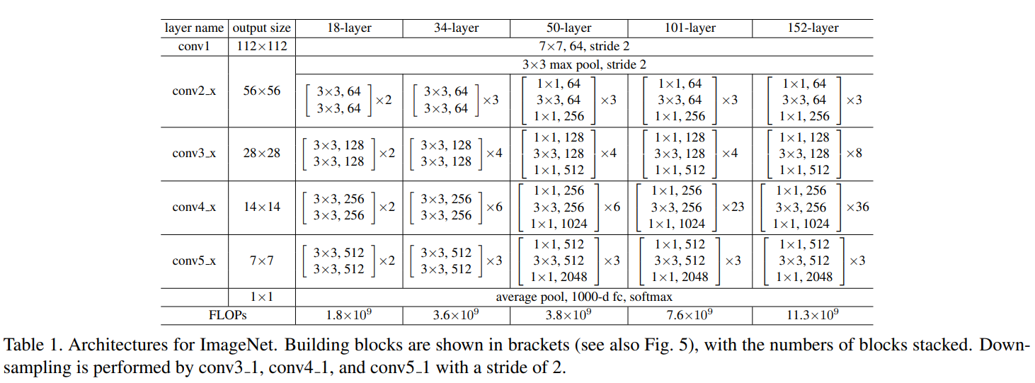
ResNet은 VGGNet처럼 \(3 \times 3\) 필터를 사용한다. \(3 \times 3\)은 공간이 지닌 특징을 하나의 값으로 추출하기 때문에 픽셀별 위치정보가 갈수록 줄어들까? 합성곱 신경망의 사이즈가 크면 한번에 많은 정보를 추출할 수 있지만, 그것보다 사이즈를 작게해서 여러 깊이(depth)로 보는게 더 낫다고 한다. ResNet에서 과적합은 주로 파마리터 수로 인해 발생한다고 주장하며, \(3 \times 3\) 필터를 거치기 전에 \(1 \times 1\)으로 깊이를 줄이고 \(3 \times 3\) 필터를 거친 후 \(1 \times 1\)으로 다시 입력 특징맵의 크기와 맞춘다.
딥러닝에서 neural networks가 깊어질수록 성능은 더 좋지만 train이 어렵다는 것은 알려진 사실입니다. 그래서 이 논문에서는 잔차를 이용한 잔차학습 (residual learning framework)를 이용해서 깊은 신경망에서도 training이 쉽게 이뤄질 수 있다는 것을 보이고 방법론을 제시했습니다.
from typing import Tuple, List, Optional, Callable

import torch
from torch import nn, Tensor
import torch.nn.functional as F


class Conv2d1x1(nn.Sequential):
    def __init__(
        self,
        in_planes: int,
        out_planes: int,
        stride: int = 1,
    ) -> None:
        super().__init__(
            nn.Conv2d(in_planes, out_planes, kernel_size=1, stride=stride, bias=False)
        )


class Conv2d3x3(nn.Sequential):
    def __init__(
        self,
        in_planes: int,
        out_planes: int,
        stride: int = 1,
        groups: int = 1,
        dilation: int = 1
    ) -> None:
        super().__init__(
            nn.Conv2d(
                in_planes, out_planes, kernel_size=3, stride=stride,
                padding=dilation, groups=groups, bias=False, dilation=dilation
            )
        )


class BasicBlock(nn.Module):
    expansion: int = 1

    def __init__(
        self,
        inplanes: int,
        planes: int,
        stride: int = 1,
        downsample: Optional[nn.Module] = None,
        base_width: int = 64,
    ) -> None:
        super().__init__()
        self.conv1 = Conv2d3x3(inplanes, planes, stride)
        self.bn1 = nn.BatchNorm2d(planes)
        self.relu = nn.ReLU(inplace=True)
        self.conv2 = Conv2d3x3(planes, planes)
        self.bn2 = nn.BatchNorm2d(planes)
        self.downsample = downsample
        self.stride = stride

    def forward(self, x: Tensor) -> Tensor:
        identity = x

        out = self.conv1(x)
        out = self.bn1(out)
        out = self.relu(out)

        out = self.conv2(out)
        out = self.bn2(out)

        if self.downsample is not None:
            identity = self.downsample(x)

        out += identity
        out = self.relu(out)

        return out


class Bottleneck(nn.Module):
    expansion = 4

    def __init__(
        self,
        in_planes: int,
        planes: int,
        stride: int = 1,
        downsample: Optional[nn.Module] = None,
    ) -> None:
        super().__init__()
        self.conv1 = Conv2d1x1(in_planes, planes)
        self.bn1 = nn.BatchNorm2d(planes)

        self.conv2 = Conv2d3x3(planes, planes, stride=stride)
        self.bn2 = nn.BatchNorm2d(planes)

        self.conv3 = Conv2d1x1(planes, planes * self.expansion)
        self.bn3 = nn.BatchNorm2d(planes * self.expansion)

        self.downsample = downsample
        self.stride = stride

    def forward(self, inputs) -> Tensor:
        residual = inputs

        outputs = F.relu(self.bn1(self.conv1(inputs)), inplace=True)
        outputs = F.relu(self.bn2(self.conv2(outputs)), inplace=True)
        outputs = self.bn3(self.conv3(outputs))

        if self.downsample is not None:
            residual = self.downsample(inputs)

        outputs += residual
        outputs = F.relu(outputs, inplace=True)

        return outputs


class ResNet(nn.Module):
    def __init__(self, layers, block=Bottleneck):
        super().__init__()
        self.num_base_layers = len(layers)
        self.layers = nn.ModuleList()
        self.channels = []

        self.inplanes = 64
        self.conv = nn.Conv2d(3, self.inplanes, kernel_size=7, stride=2, padding=3, bias=False)
        self.bn = nn.BatchNorm2d(self.inplanes)
        self.relu = nn.ReLU(inplace=True)
        self.maxpool = nn.MaxPool2d(kernel_size=3, stride=2, padding=1)

        self._make_layer(block, 64, layers[0])
        self._make_layer(block, 128, layers[1], stride=2)
        self._make_layer(block, 256, layers[2], stride=2)
        self._make_layer(block, 512, layers[3], stride=2)

    def _make_layer(self, block, planes, blocks, stride=1):
        downsample = None
        if stride != 1 or self.inplanes != planes * block.expansion:
            downsample = nn.Sequential(
                Conv2d1x1(
                    self.inplanes,
                    planes * block.expansion,
                    stride=stride,
                ),
                nn.BatchNorm2d(planes * block.expansion)
            )

        layers = [block(self.inplanes, planes, stride, downsample)]
        self.inplanes = planes * block.expansion

        for _ in range(1, blocks):
            layers.append(block(self.inplanes, planes))

        self.channels.append(planes * block.expansion)
        self.layers.append(nn.Sequential(*layers))

    def forward(self, inputs):
        inputs = self.conv(inputs)
        inputs = self.bn(inputs)
        inputs = self.relu(inputs)
        inputs = self.maxpool(inputs)

        outputs = []
        for layer in self.layers:
            inputs = layer(inputs)
            outputs.append(inputs)

        return outputs


def resnet18():
    backbone = ResNet([2, 2, 2, 2], BasicBlock)
    return backbone


def resnet34():
    backbone = ResNet([3, 4, 6, 3], BasicBlock)
    print(backbone.channels)
    return backbone


def resnet50(pretrained: bool = False):
    backbone = ResNet([3, 4, 6, 3], Bottleneck)
    return backbone


def resnet101(pretrained: bool = False):
    backbone = ResNet([3, 4, 23, 3], Bottleneck)
    return backbone
실험결과#

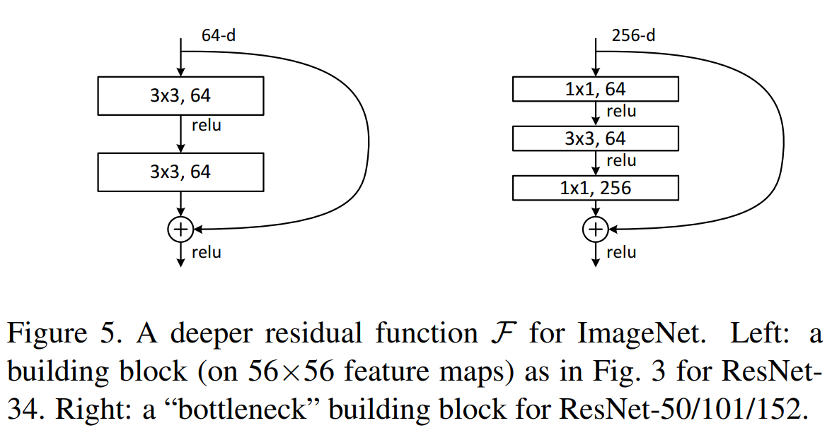
ResNet 연구팀은 bottleneck design을 ResNet-50/101/152에 적용했다. 차원이 깊어짐에 따라 연산량이 많아져 학습시간이 길어지기 때문에 기본 블록을 병목 블록으로 두 개의 레이어를 세 개의 레이어로 쌓아 병목 구조의 블록을 고안하였다. 깊이는 깊어지나 시간복잡도(time complexity)가 비슷하고 Identity shortcut 사용되며 projection 사용시 model 복잡도와 size가 2배로 증가한다